About RTXI

The Real-Time eXperiment Interface (RTXI) is a collaborative open-source software development project aimed at producing a real-time Linux based software system for hard real-time data acquisition and control applications in biological research. RTXI merges three previous systems for closed-loop biological experiments: RTLab, Real-time Linux Dynamic Clamp (RTLDC), and Model Reference Current Injection (MRCI). RTLDC and MRCI focus on implementing dynamic clamp, an experimental technique in cardiac and neural electrophysiology that is used to simulate ionic membrane currents. RTXI combines the features of all three predecessor platforms into a more general platform for real-time closed-loop experimental protocols. Using real-time control, scientists can quantify biological function via perturbations that change according to closed-loop analysis of measured system variables, rather than being restricted to measuring responses to pre-determined stimuli. Real-time control applications are abundant throughout biological research, including, for example, dynamic probing of ion-channel function, control of cardiac arrhythmia dynamics, and control of deep-brain stimulation patterns. There is a wide range of biological research endeavors for which real-time control can offer insight that cannot be obtained with traditional methods.

RTXI is based on Linux, which is extended with Xenomai to provide a hard real-time platform with the comprehensive Linux desktop environment. Data acquisition and analog/digital interfaces to other hardware are implemented in real-time using the Analogy real-time driver interface, which provides support to a variety of commercial multifunction data acquisition cards. Experimental protocols and other real-time algorithms are implemented within a modular framework that allows users to easily reuse existing code and construct complex protocols. Users can also take advantage of previously written code or other cpp libraries to add functionality to their modules. As such, RTXI is a generic real-time platform with potential applications beyond dynamic clamp.

RTXI is released under a combination of the GPL and LGPL licenses. The core RTXI code is covered by a GPL license but user modules distributed as binary libraries are covered under LPGL and their source code may be available at the discretion of the original authors. All documentation is released under the GNU Free Documentation License.

If your use of RTXI leads to scientific publication, we request that you cite RTXI in your paper with text such as:

Overview

RTXI contains many features that enable users to quickly implement complex interactive experimental protocols:

• Modular signal-and-slots architecture that allows multiple instantiations of user modules, makes it easy to reuse code such as event detection and online analysis algorithms, and allows branching logic so that signals (such as acquired data) can be routed through multiple algorithms in parallel
• Data acquisition system that can stream multiple channels of acquired or computed data along with experimental metadata and user comments with timestamps
• Ability to interface with a variety of multifunction DAQ cards and external hardware through analog or digital channels, e.g. via TTL pulses
• Ability to change experimental parameters on-the-fly without recompiling or stopping real-time execution
• Ability to save and reload your entire working environment with custom parameter settings
• Virtually no limit to algorithms that can be implemented since user modules are written in cpp
• Real-time digital oscilloscope that can plot any acquired or computed signal
• Base class for constructing user modules with a customized graphical user interface to experimental protocols
• Ability to 'play back' previously acquired data or surrogate data as if it were being acquired in real-time for debugging or simulation purposes
• A complete simulation platform that can be used to solve systems of differential equations in real-time and integrate biological signals acquired in real-time with model systems

In addition, RTXI is available on a Live CD, which provides a complete real-time Linux operating system with RTXI without installing anything on your computer. This live environment allows you to mount your existing hard drive and you can conduct experiments and collect data. Note that the real-time performance will be slower compared with an actually installed system. Running the live environment from a USB flash drive is faster than from an actual CD. A DAQ card does not need to be installed for RTXI to run and RTXI can be successfully run on many laptops, including Intel MacBooks and MacBook Pros.

Introduction to Dynamic Clamp

Traditionally, the properties of electrically excitable cells are assessed using current clamp and voltage clamp electrophysiology protocols. In current clamp, an electrical current waveform is specified and applied to the cell through a microelectrode while the transmembrane potential is recorded. In voltage clamp, a desired voltage waveform is specified and analog circuitry is used to determine and inject a current that is necessary to maintain, or clamp, the membrane potential at the specified values. The dynamic clamp allows the insertion of artificial membrane conductances, such as ion channels, by injecting current that is a function of the cell's membrane potential. The injected current is computed by computer software or analog circuitry based on the equivalent circuit model of an excitable cell (Fig. \ref{fig:circuit}). The artificial conductance is effectively in parallel with other membrane processes, each of which contributes to the total transmembrane current.

The total transmembrane current is related to changes in the membrane potential, V_m, through the following equation:

where C_m is the membrane capacitance. Any conductance that can be described mathematically can be applied to a neuron using the dynamic clamp. The current passing through an ion channel, for example, is often described by Ohm's law using the following conductance-based equation:

where g is the maximal conductance, and m and h are voltage-dependent activation and inactivation gating variables (p and q are integers) that describe the kinetic activation of the channel. Gating variables have values between 0 and 1 to scale the channel conductance and are typically described by a first order differential equation:

The membrane potential is re-sampled and the equations are re-evaluated on every computational cycle of the dynamic clamp system. As such, the dynamic clamp is also sometimes termed conductance clamp or conductance injection.

While the dynamic clamp was first demonstrated in cardiac electrophysiology to electrically couple embryonic chick myocytes, the technique was independently introduced ( Robinson, 1993 and Sharp, 1993) and is now more prevalent in neural electrophysiology ( Economo, 2010; Prinz, 2014; and Goaillard, 2006). Applications of this technique include the insertion of non-native ion channels (a virtual "knock-in"), subtraction of native ion channels (a virtual "knock-out"), and simulation of synapses and electrical gap junctions to create small networks of biological and/or simulated neurons. By varying the parameter values of a model channel or synapse, experiments can be conducted to determine how these properties shape membrane dynamics and neuron activity. These approaches have made the dynamic clamp a valuable tool for studying the intrinsic properties of single neurons and the behavior of small neural networks.

Dynamic clamp studies have also made important contributions to our understanding of neuronal dynamics under in vivo-like conditions in which neurons receive a constant barrage of synaptic inputs which can easily reach thousands of events per second. Artificial synaptic input can be constructed from pre-recorded activity of presynaptic neurons but is more commonly based on statistical descriptions of noisy conductance waveforms. This high conductance state has been shown to enhance the cell's responsiveness to small inputs, also known as its gain ( Chance, 2002; Destexhe, 2003; and Sceniak, 2010), and can change the signal integration of synaptic input, creating distinct modes of firing patterns (Wolfart, 2005; Steriade, 2001; Rudolph, 2003; and Destexhe, 2001). The statistics of current-based versus conductance-based input, such as correlations and relative balance between excitation and inhibition, are translated differently into output statistics such as the membrane potential distribution, the distribution of interspike intervals (ISIs), the coefficient of variation (CV), and the mean and variance of the neuron's output firing rate (Tiesinga, 2000; Rudolph, 2003; Kumar, 2008; and Salinas, 2000). Together, these factors result in a dynamical behavior of the neuron that is usually quite different from the intrinsic dynamics of the voltage-gated currents.

Results from dynamic clamp experiments must be carefully interpreted due to several experimental limitations. Space-clamp problems arise in that the injected current is limited to a space around the recording electrode. In some experimental studies, an artificial dendrite is modeled as well to simulate the cable effects of synaptic inputs propagating to the action potential initiation zone (Hughes, 2008). Since current can usually only be injected at the soma, the dynamic clamp may be a poor approximation of dendritic input in some cell types. In most cells, the dynamic clamp is operated in discontinuous current clamp (DCC) mode in which a single electrode switches between recording and current injection states. In this configuration, it is not possible to inject large conductances that approach the magnitude of the cell's intrinsic resting conductance while still accurately recording the membrane potential. The injected current induces a voltage drop through the electrode and causes measurement accuracies that are propagated through the closed feedback loop in the dynamic clamp system and may cause ringing artifacts in the recording ( Brizzi, 2004; Jaeger, 1999; Preyer, 2007; and Preyer, 2009). In larger cells, two electrodes may be used, one to record and one to inject current. Researchers also typically use the same ion channel or synapse model parameters for all cells used in an experiment, assuming that neurons of the same cell type have identical intrinsic properties, both within an animal and between animals ( Golowasch, 2002). There usually is not time during an experiment to manually adjust the model to optimal parameters for each cell.

Compared to other real-time closed-loop experimental protocols, the dynamic clamp has perhaps the most stringent performance requirements. These limitations involve numerical, algorithmic, and hardware platform-specific issues. Dynamic clamp performance depends on how accurately the model is solved, measurement error in sampling the voltage, and the sampling rate of the system. \index{sampling rate}The sampling rate determines how much time is in a given computational cycle for various operations to be performed, and the duration of the cycle restricts the types of numerical methods that may be used to integrate the gating variables. Thus, the computational performance of dynamic clamp suffers from a trade-off between the speed of computation and numerical accuracy. Dynamic clamp sampling rates are currently chosen based on the limits of the hardware platform being used and the temporal dynamics being simulated. While it is possible to compute the time step necessary for the Euler and exponential Euler methods to achieve a desired one-step integration accuracy for a known voltage measurement error, few studies employ this technique (Butera, 2004). In simulations of dynamic clamp, Euler integration was insufficient to model fast sodium Na_v channels at sampling rates under 30 kHz and nearly identical integration results for three different deterministic integration methods was only achieved at rates >=50 kHz (Milescu, 2008). Standard performance benchmarks are needed for dynamic clamp to justify the sampling rates that are used.

Other hardware that are typically required for dynamic clamp are an electrophysiology amplifier for measuring membrane potential and injecting current and a multifunctional data acquisition system (DAQ) for performing analog-to-digital (ADC) and digital-to-analog (DAC) conversion. The technical specifications of each of these hardware components can affect the performance of the overall system by introducing additional jitter, latency, and quantization error that can affect system timing and the numerical computation (Bettencourt, 2008 and Butera, 2001). Recent results show that faster systems would result in a greater range of conductances that could be utilized, improved stability, and more accurate real-time model simulations (Preyer, 2007 and Preyer, 2009). Faster dynamic clamp systems have been developed, largely due to the increasing power of personal computers, but also due to the development of systems based on the GNU/Linux operating system and embedded real-time processors.

Hardware Requirements

RTXI is designed to run on a standard personal desktop computer. Computers with uniprocessors, multi-core processors, and multiple CPUs with and without hyperthreading are supported by Linux and RTXI, though typically more stable systems are realized with Intel rather than AMD processors. For multi-core computers, Xenomai will need to be manually configured during installation. In rare cases, a particular CPU and motherboard combination is not supported. Certain advanced motherboards may contain features that are not compatible with Xenomai, such as some integrated graphics chips that use hardware-level techniques to speed up computation. For video cards, we recommend you use an external one. Generally, NVIDIA cards have better Linux support than ATI/Radeon ones. This distinction is important because the greatest overhead in RTXI is related to data visualization in the oscilloscope. For newer graphics cards, you may need to manually install the Linux drivers, usually available on the manufacturer's website. Some systems may also include BIOS level or hardware interrupts that are not captured by Xenomai or advanced power management features. Sometimes these can be disabled by the user in the BIOS.

The real-time Linux kernel has extremely low latencies and little software overhead. RTXI is also designed to minimize the number of dynamically loaded modules and keep overhead low. RTXI has been successfully tested on computers with Pentium III processors up to 4(8)-core Intel i7 processors. While the processor speed allows RTXI to complete more computations within a single real-time cycle, the amount of RAM and the amount of video memory have a significant impact on the stability and speed of the system. Users should also consider high speed hard drives, large cache sizes, and high speed bus interfaces. If you are purchasing an off-the-shelf desktop computer system and plan to add a DAQ card, be sure that your power supply is powerful enough to handle the extra load. At least a 450W power supply is recommended.

Data Acquisition Cards

For closed loop experiments using RTXI, your computer must be equipped with an analog-to-digital converter (ADC) to acquire data and a digital-to-analog converter (DAC) to generate signals. Of course, external hardware such as an oscilloscope or function (waveform) generator can be used in conjunction with RTXI. A popular option is to purchase a commercial multifunction data acquisition card that provides analog input and output, digital input and output, and counter/timer circuitry. DAQ cards using the USB interface are not compatible with RTXI because USB drivers in Linux are not capable of hard real-time operation. Furthermore, the USB interface can only achieve a maximum sampling rate of approximately 1 kHz, insufficient for some closed-loop real-time applications. Many DAQ cards using the PCI, PCI express, or PXI interface are available from a variety of manufacturers. Your choice of DAQ card should depend on the number of analog and/or digital channels that you need, the amount of data resolution (eg. 12, 16-bit), sampling resolution, speed, and whether you need simultaneous or sequential sampling of multiple input channels.

Most RTXI users use products developed by National Instruments. ANALOGY, a set of drivers derived from ANALOGY, provides support for many NI DAQs, for low-level drivers for cards using a 8255 chip for three channels of 8 bit digital input or output, and for standard PC parallel ports. A list of currently supported NI cards and their corresponding ANALOGY driver and other ANALOGY-supported DAQ manufacturers is given below.

Adding more DAQ cards

RTXI has no built-in software limitations on the number of DAQ cards but is configured for only one card by default. If you want to use additional cards, you will need to edit the configuration file. Here is the relevant excerpt of /etc/rtxi.conf:

<OBJECT component="plugin" library="analogy_driver.so" id="2">
<PARAM name="0">/dev/analogy0</PARAM>
<PARAM name="Num Devices">1</PARAM>
<OBJECT id="13" name="0" />
</OBJECT>

Edit the lines to add another ANALOGY device and change the number of devices:

<PARAM name="0">/dev/analogy0</PARAM>
<PARAM name="1">/dev/analogy1</PARAM>
<PARAM name="Num Devices">2</PARAM>

You will need to exit and restart RTXI for the new configuration to take effect. Settings files that you have already created should still work when you change rtxi.conf but you may not have access to both DAQ cards in the System Control Panel, the Oscilloscope, and the Connector. You will have to rebuild those settings files or edit them as above using your choice of text editor.

RTXI automatically detects the manufacturer and board names of available DAQ cards and the number and type of input and output channels. The first DAQ card installed in your system is assigned the Linux device name: /dev/analogy0. Additional DAQ cards are assigned device names /dev/analogy1 and so on. You can check that your DAQ card has been correctly detected and see the corresponding device name by clicking Help --> About ANALOGY from the RTXI menu bar.

Real-time Performance

Xenomai provides several command line utilities for testing your real-time performance. These are available in your Xenomai installation directory at /usr/xenomai/bin). There are both user and kernel space versions of the available tools. When using these tests, keep in mind that they are most informative when the system is under processing loads, ideally loads similar to those added when you run RTXI.

The most important test is the latency test. It measures the latency, or the difference in time between the expected switch time and the time a task is actually called by the scheduler. It is essentially a measure of the delay when a task is supposed to run and when it actually runs. For a system to run in real-time, the latency values must be below the frequency at which a task must be run. For example, to run something in real-time at 20 kHz, the latencies must remain below 50 us. Failure to do so constitutes an overrun.

The latency test will perform latency calculations repeatedly (default 10 kHz) until stopped. To run, go to the /usr/xenomai/bin directory and execute: $ sudo ./run. To stop a running test, use CTRL-C in the terminal.

== Sampling period: 100 us
== Test mode: periodic user-mode task
== All results in microseconds
warming up...
RTT|  00:00:01  (periodic user-mode task, 100 us period, priority 99)
RTH|----lat min|----lat avg|----lat max|-overrun|---msw|---lat best|--lat worst
RTD|     -2.376|     -2.185|     -0.114|       0|     0|     -2.376|     -0.114
RTD|     -2.721|     -2.171|      0.100|       0|     0|     -2.721|      0.100
RTD|     -2.725|     -2.175|      1.223|       0|     0|     -2.725|      1.223
RTD|     -2.363|     -2.185|      0.416|       0|     0|     -2.725|      1.223
RTD|     -2.720|     -2.193|     -0.584|       0|     0|     -2.725|      1.223
RTD|     -2.527|     -2.144|      5.550|       0|     0|     -2.725|      5.550
RTD|     -2.272|     -2.193|     -1.120|       0|     0|     -2.725|      5.550
RTD|     -2.716|     -2.193|     -0.455|       0|     0|     -2.725|      5.550

The test prints one line every second and gives you the minimum, average, and maximum latencies for that period as well the minimum and maximum overall latencies that occurred over the entire test. Open up some other programs, copy some files from one location to another, and load the network connection to see how it affects the latency. The system's real-time performance is limited by the maximum latency (the 'lat worst' column). You should not any overruns, meaning that the latency completely exceeds the nominal period. Negative time values in the latency test is due to the fact that Xenomai performs a calibration at startup that tries to minimize the jitter in the real-time task and anticipates the call. You can correct this behavior by running (as root):

# echo 0 > /proc/xenomai/latency

There are many factors that affect your real-time performance, which do not necessarily depend on your absolute processor speed. For simple applications such as a single ion channel, similar results can be obtained on 200 MHz or 2 GHz processors. The limiting factors actually involve the design of the motherboard and chipset, the cost of reading and writing to a DAQ card, and the cost of accessing the hard disk when streaming data. Multi-processor systems or multicore processors also operate differently than single processors. RTXI allows the system to distribute processes among individual cores and does not assign any operations to particular cores. The user can use the isolcpus and xeno_hal.supported_cpus boot options to limit real-time operations to a single core and let all other non real-time operations be distributed among other available cores. Generally, you'll get the best RT performance from your system if you disconnect from your network, especially if is a wireless network, and to plot only the minimum number of signals in the Oscilloscope module as possible.

If you periodically see an overrun (perhaps every 64 seconds) that results in a maximum latency of several hundred microseconds, you may have an SMI (System Maintenance Interrupt) issue. This feature can be found on certain chipsets e.g. Intel 82845 845. Disabling SMI can cause some computers to overheat and may damage those computers. Other latency killers are: heavy DMA activities (using the hard disk), using an accelerated Xserver, USB legacy support, power management (APM and ACPI), and CPU frequency scaling. If you have disabled all of these in the kernel already, check your BIOS and see if you can disable them there.If you installed RTXI using our Live CD or installation instructions, these are already correctly configured.

RTXI Menu

Although RTXI is dependent on Linux, it is a complete desktop application and configuration of system settings and interaction with most features are available through a graphical user interface.

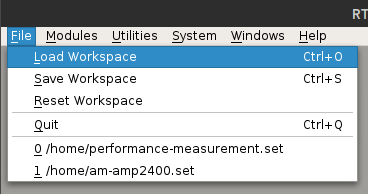
The File Menu is used to save and load settings files that capture the entire working environment. This includes settings configured in the System Control Panel, such as channel gains, parameters set within modules, and connections between modules. Reloading a settings files will also restore the window sizes and positions at the time the file was created. Recently used settings files are also available from this menu.

The Modules Menu is used to load user modules. User modules are shared libraries that are installed to /usr/local/lib/rtxi during the compilation process. Choosing "Load User Module" opens a file dialog box at this location, from where users may select modules based on the *.so filename.

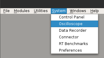
The System Menu is used load core RTXI system features and modules. The Control Panel is used to configure channels and set the nominal system period (or sampling rate). The Oscilloscope is the digital oscilloscope that can be used to plot any signal in real-time. The Data Recorder allows users to select signals to stream to a HDF5 file in real-time. The Connector is used to specify connections between modules and the DAQ card. The Performance Measurement module displays running statistics on the computational load in RTXI. There is also a Preferences panel for specifying commonly used directories, etc.

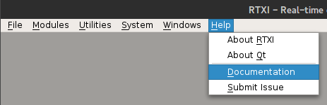
The Help Menu contains important information about your system and RTXI. You can view the version number of your RTXI installation and the version of Qt used to build the user interface. Also included is a link to our documentation website and a link to our GitHub repository where you can report any issues you have with your system.

Core System Modules

The following modules are included in RTXI by default and are available through the System menu. All settings edited in each of these modules can be saved and reloaded via workspaces. Save by choosing File --> Save Workspace from the RTXI menu bar. This will create a basic *.set file that you can load in the future to recreate this environment or use as a foundation for additional *.set files.

System Control Panel

The System Control Panel allows you to set important parameters on all the input and output channels of your DAQ card and set the nominal real-time period of your system. To keep the number of RT events to a minimum, all changes made in the Control Panel are not set until the Apply button is pressed.

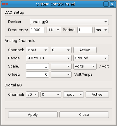
DAQ Setup

RTXI automatically detects the manufacturer and board names of available DAQ cards and the number and type of input and output channels. The first DAQ card installed in your system is assigned the Linux device name: /dev/analogy0. Additional DAQ cards are assigned device names /dev/analogy1 and so on.

You can use either the Frequency or Period entry boxes to set the real-time period. After you enter the value, hit Apply to set your changes.

Analog
Channels

The Channel submenu lists all avaiable analog input and output channels for the specified DAQ device. Picking a particular channel will allow you to activate the channel and also set the parameters of that channel via the Range, Scale, and Offset menus below. To activate a channel (i.e. tell the DAQ driver to start reading/writing the channel), press down the Active button, and then hit Apply.

NOTE: If you do not hit the Apply button before changing channels, all changes made , such as the range, activation state, etc. will be lost.

The Range, Scale, and Offset submenus set the acquisition range and the reference mode. By default, RTXI assumes that all analog DAQ input and output channels have a range from -10 V to +10 V, unity gain (or a scaling of 1 V/V), a 0 V offset, and a ground reference. You must set the correct options for each channel you are using to acquire and output the correct signal values. Remember to hit Apply to set your changes.

Digital I/O

If you DAQ supports digital I/O, use this section of the control panel to activate individual channels. All you need to do is set whether the channel is to an input or an output, hit the Active button, and the hit Apply. For digital outputs, RTXI will output 0 V when 'false' and 5 V when 'true'.

Oscilloscope

The Oscilloscope allows you to plot any system signal, such as signals from/to the DAQ card and signals from user modules. Each signal may have a different vertical scale and line style and a legend is automatically generated in the Oscilloscope window.

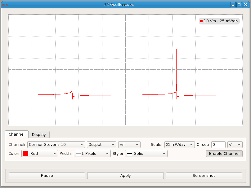
Channel

Select signals to plot from the dropdown menu. You can plot any input or output from a loaded module or active channel on your DAQ. DAQ signals will appear as an ANALOGY source, eg. analogy0. Be sure to check whether you have to set additional settings in the System Control panel to compensate from gains from any additional instrumentation. Input to the DAQ card from external instrumentation, such as an external amplifier, is designated as output from the DAQ card within RTXI. RTXI will automatically detect how many input and output channels your card has. Signals from other modules will be identified by the module name and you can choose from any inputs, outputs, parameters, or states that are defined in those modules.

Use the Scale and Offset options to modify the signals being plotted. To actually plot the signal, you must depress the Active toggle button and hit Apply. Any modifications you make to the scaling, offset, or line style of the signal are not active until you hit Apply again. Note that plotting too many signals in real-time may affect your system performance and cause your GUI to freeze during program execution. Use the RT Performance module to watch the load on your system while the Oscilloscope is running.

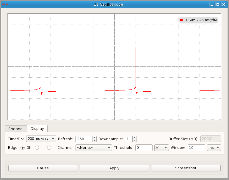
Time/Div

Use the dropdown menu to set the time scale for the x-axis. Each "div" refers to the demarcations on the plot window. You can also set the refresh rate, or the number of times the plot window is refreshed per second, and you can set a downsampling rate for plotting.

Edge

Use the Edge option to set a trigger to freeze the oscilloscope when certain criteria are met by a specified channel. Set the trigger to operate on a rising or falling edge by clicking the + or - radio buttons, respectively. The Channel can be set to any active signal that is currently plotted on the oscilloscope. Threshold sets the threshold for the trigger channel you specified, and Window sets the amount of time that lapses before the trigger is reset again. The trigger threshold is indicated on the oscilloscope by a horizontal yellow dashed line.

To start the trigger, set everything in the menu and then hit the Apply button. To stop, select the Off radio button and hit Apply again.

Data Recorder

The Data Recorder module allows users to stream synchronous data to a HDF5 file. Open the module by selecting System --> Data Recorder from the RTXI menu bar.

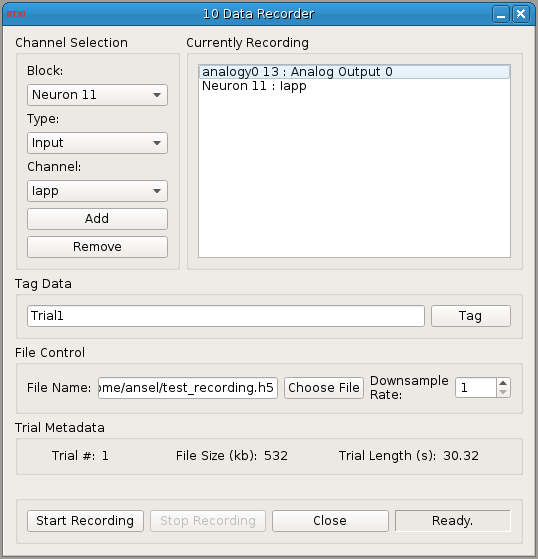
Channel
Selection

The Block menu is a list of your DAQ card(s) and any loaded user modules. Selecting a block device then populates the Type and Channel menus. Navigate the menus until you specify the channel you want to record. Then, hit Add to add the channel to the Currently Recording block. To remove a channel from the list, double-click its name in the list and then press the Remove button.

File Control

Before you can start recording, you must select a file by clicking the Choose File button. Navigate to the directory where you want to save you file. From the menu, you can either create a new HDF file select an existing one. If you choose the latter, you can either append new data to the file, preserving any existing data, or you can simply overwite it, erasing any existing data and only saving new trials.

Click Start Recording to begin recording and Stop Recording to stop recording. For each module connected to the Data Recorder, it also grabs all the parameter values and saves them as metadata. In addition, it logs when any of these parameter values change so that you have a complete record of your experiment.

If you have a configuration such that Module A: Output 0 --> Module B: Input 0, saving Output 0 from Module A and Input 1 from Module B will give you exactly the same data. Similarly, saving /dev/analogy0: Analog Output 0 will save the signal that has been assigned to that channel (perhaps generated by a user module), not the actual signal the DAQ card is outputting. To check the actual output of the DAQ card, you will need to make a connection from that output to another input channel.

Trial Metadata

Each time you start and stop the data recorder counts as one 'trial'. By default, the Data Recorder displays the current trial number, the size of your data file, and the length of time from your last trial. "Trials" have to do with the data structure heirarchy within the HDF files. More information on what that means is provided below.

Connector

The Connector module allows you to create data streams between modules or between modules and the DAQ card.

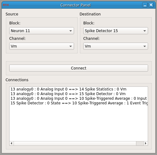
Source

The Source block displays all Input channels from your DAQ and all OUTPUT variables from any open modules. The name of each module and analogy device is displayed in the Block drop-down menu, and the name of each analog/digital input channel or module output channel is displayed in Channel.

RTXI automatically detects how many inputs are available on your DAQ card. Note that the module does not check whether the channels are enabled via the Control Panel.

Destination

The Destination block displays all Output channels on your DAQ and all INPUT variables from any open modules. The name of each module and analogy device is displayed in the Block drop-down menu, and the name of each analog/digital output channel or module input channel is displayed in Channel.

Connections

To connect one module from the other, select the desired Source and Destination channel. Then, click Connect. Now, every real-time period, the value of the Source channel is read in as input for the Destination channel.

All active connections are listed in the Connections box. To remove an existing connection, double-click on its entry in the list and again click the Connectbutton.

Real-time Benchmarks

The RT Benchmarks module gives you timing statistics for RTXI. For hard real-time performance, all operations must complete within the nominal system period. This module continuously keeps track of the time needed to complete these tasks, as well as the actual real-time period. In addition, the module reports the worst case total computation time and the worst case time step for however long the module was openor the statistics were last reset.

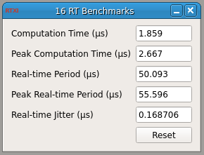
Comp Time

The time it takes for all RT components (system modules + execute loops from user modules) to run in a single RT cycle.

Peak Comp
Time

The peak computation time measured over the time the RT Benchmarks module was running or was last reset.

RT Period

The timestamp of the current RT period minus the timestamp from the last period. Basically, a measure of how long the previous period lasted. Ideally, this number is very close to the nominal RT period set in the Control Panel.

Peak RT
Period

The maximum RT Period measured over the time the RT Benchmarks module was running or was last reset.

RT Jitter

The standard deviation of all the real-time periods measured over the time since the RT Benchmarks module was opened or last reset.

User Modules

RTXI comes with a set of core system modules but also enables users to install custom modules. All modules are compiled as Linux shared object libraries (*.so) that are linked into the core system. This allows RTXI to have minimal overhead and user modules are loaded only as needed. This architecture also allows multiple instantiations of user modules so that elements such as filters and event detectors can be reused on a variety of signals.

The compilation and installation process will create an RTXI shared object library (*.so extension) in /usr/local/lib/rtxi, where RTXI will initially look for them. User modules must be recompiled if any changes are made to their sources after installation. Note that when reinstalling modules, the corresponding *.so files are overwritten, so always make sure that different modules have unique names.

DefaultGUI and the Plugin Template

This is an explanation for the code found in the plugin template module and a brief introduction to the DefaultGUI framework it abstracts. The plugin template contains starter code for building new RTXI modules, though you can fork any other module, too. Below are the contents of plugin-template.cpp and plugin-template.h. Click on a code block to display an explanation of how its code works. If anything is unclear, let us know.

This tutorial will assume the reader has a basic understanding of C++, such as including libraries and source files, classes, inheritance, etc. For a quick run-down of C++ for people already familiar with programming, this is a decent place to start.

plugin-template.h

/*
 * This is a template header file for a user modules derived from
 * DefaultGUIModel with a custom GUI.
 */

#include <default_gui_model.h>

class PluginTemplate : public DefaultGUIModel {

   Q_OBJECT

   public:

      PluginTemplate(void);
      virtual ~PluginTemplate(void);

      void execute(void);
      void customizeGUI(void);

   protected:

      virtual void update(DefaultGUIModel::update_flags_t);

   private:

      double some_parameter;
      double some_state;
      double period;

      void initParameters();

   private slots:
   // these are custom functions that can also be connected
   // to events through the Qt API. they must be implemented
   // in plugin_template.cpp

      void aBttn_event(void);
      void bBttn_event(void);

};

plugin-template.cpp

/*
 * This is a template implementation file for a user module derived from
 * DefaultGUIModel with a custom GUI.
 */

#include <plugin-template.h>
#include <main_window.h>
#include <iostream>

extern "C" Plugin::Object *createRTXIPlugin(void){
   return new PluginTemplate();
}

static DefaultGUIModel::variable_t vars[] = {
   { "GUI label", "Tooltip description", DefaultGUIModel::PARAMETER
      | DefaultGUIModel::DOUBLE, },
   { "A State", "Tooltip description", DefaultGUIModel::STATE, },
};

static size_t num_vars = sizeof(vars) / sizeof(DefaultGUIModel::variable_t);

PluginTemplate::PluginTemplate(void) : DefaultGUIModel("PluginTemplate with Custom GUI", ::vars, ::num_vars) {
   setWhatsThis("<p><b>PluginTemplate:</b><br>QWhatsThis description.</p>");
   DefaultGUIModel::createGUI(vars, num_vars); // this is required to create the GUI
   customizeGUI();
   initParameters();
   update( INIT ); // this is optional, you may place initialization code directly into the construct    or
   refresh(); // this is required to update the GUI with parameter and state values
   QTimer::singleShot(0, this, SLOT(resizeMe()));
}

PluginTemplate::~PluginTemplate(void) { }

void PluginTemplate::initParameters(void) {
   some_parameter = 0;
   some_state = 0;
   return;
}

void PluginTemplate::execute(void) {
   return;
}

void PluginTemplate::update(DefaultGUIModel::update_flags_t flag) {
   switch (flag) {
      case INIT:
         period = RT::System::getInstance()->getPeriod() * 1e-6; // ms
         setParameter("GUI label", some_parameter);
         setState("A State", some_state);
         break;

      case MODIFY:
         some_parameter = getParameter("GUI label").toDouble();
         break;

      case UNPAUSE:
         break;

      case PAUSE:
         break;

      case PERIOD:
         period = RT::System::getInstance()->getPeriod() * 1e-6; // ms
         break;

      default:
         break;
   }
}

void PluginTemplate::customizeGUI(void) {
   QGridLayout *customlayout = DefaultGUIModel::getLayout();

   QGroupBox *button_group = new QGroupBox;

   QPushButton *abutton = new QPushButton("Button A");
   QPushButton *bbutton = new QPushButton("Button B");
   QHBoxLayout *button_layout = new QHBoxLayout;
   button_group->setLayout(button_layout);
   button_layout->addWidget(abutton);
   button_layout->addWidget(bbutton);
   QObject::connect(abutton, SIGNAL(clicked()), this, SLOT(aBttn_event()));
   QObject::connect(bbutton, SIGNAL(clicked()), this, SLOT(bBttn_event()));

   customlayout->addWidget(button_group, 0, 0);
   setLayout(customlayout);
}

The customizeGUI function is designed for users to customize the default UI output created by the DefaultGUIModel class. The initial module is created by the createGUI function called above in the constructor. Broadly speaking, this function takes the output of createGUI and adds custom elements to it. To use this function, you will need to know what the Qt classes are and how to use them properly. Documentation is available on the Qt website. (http://doc.qt.io/qt-5.5/)

To customize the module UI, it first needs to be grabbed and stored in a variable, which is accomplished in the first line of the function. DefaultGUIModel::getLayout() returns an object of type QGridLayout. This essentially is a widget that allows Qt objects to be aligned according to a grid layout. The layout of DefaultGUIModel is as follows:

By default, the main UI is displayed within the grid at coordinates (1,0) and the utility box with the pause, modify, and exit buttons at coordinates (10,0). All other positions on the grid are empty.

Note that the size of grid coordinates are arbitrary. They are as big as the widgets that are stuck within them. They're equally-sized in the diagram just for clarity. Look through Qt's documentation for instructions on how to set widgets at specific positions in the grid layout.

Also, note that coordinates that are empty are not rendered, so there is no big gap between the Main UI and the Button UI because there is nothing put in spots (2,0) to (9,0). Keep in mind, though, that the QGridLayout will not allow objects in diffrent rows to overlap. For example, if you added an object to (1,5), the UI in (0,1) would render, followed by a gap the size of the widget in (1,5), and then the buttons in (0,10). The object in (1,5) would be shown in column 1.

The rest of the code in customizeGUI creates two buttons and sticks them into coordinate (0,0). The buttons are then connected to functions using Qt's signals and slots API. When a button is pressed, it emits a signal that it has been pressed, and the connect connects that signal to a function. The effect is then to call the function whenever the button is pressed.

When all the modifications are complete, they need to be added to the module layout that was grabbed by DefaultGUIModel::getLayout(). This is done using the setLayout command.

// functions designated as Qt slots are implemented as regular C++ functions
void PluginTemplate::aBttn_event(void) { }

void PluginTemplate::bBttn_event(void) { }

HDF5 Data Files

The HDF5 file format is a portable and extensible binary data format designed for complex data. It supports an unlimited variety of datatypes and flexible and efficient methods for data retrieval and storage. HDF5 features a hierarchical structure that allows access to chunks of data without loading the entire file into memory. The Data Recorder module outputs to an HDF5 file.

At the topmost level, an RTXI HDF5 file is divided into separate Trial groups, each of which contains the system settings and module parameter values that existed at the time that data was recorded. The Data Recorder only saves parameter values for modules from which it is recording a signal. A new Trial is created whenever the Data Recorder is used to start recording. For example, if you stop and start recording multiple times in a single session, RTXI automatically increments the trial number each time. If you choose to save data to a file that already exists, RTXI will prompt you with a choice to overwrite the file or append new data to the file. Appending data to a file also creates a new Trial. Thus, it is possible to have trials within the same file that contain different parameter settings and even data downsampling rates.

Parameter values from user modules are saved in the Parameters group within each Trial. The name of each parameter includes the module instance ID number within RTXI, the name of the module, and the name of the parameter itself. If the value of the parameter changes during recording, all the values are saved with a corresponding index value that is the timestamp in nanoseconds from the start of the recording. This feature is only available for user modules that are based on the DefaultGUIModel class. Note that certain naming conventions for parameters also apply in order for them to be captured to HDF5.

Real-time signals in RTXI are streamed to the Synchronous Data structure within each Trial. This group contains separate fields with the name of each synchronous channel and a single dataset that contains all the synchronous data. The order of the channel names corresponds with the columns in the dataset.

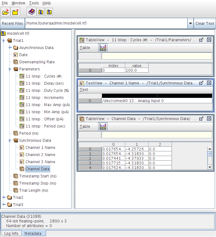
There are various software available for working with HDF5 files. To simply browse the file structure, you can use the free HDFView application:

$ sudo apt-get install hdfview

HDFView provides some limited editing capabilities. For trials where only a single channel is saved, you can also preview a plot of the data. To extract the data for analysis and for complete editing capabilities, APIs are available for MATLAB, GNU Octave, Igor Pro, Mathematica, Python, Scilab, and other software.

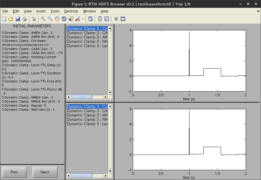
RTXI also includes a simple MATLAB GUI for quickly viewing the data within a single trial. The MATLAB code is available in the Analysis Tools repository. A sample m-file called example.m provides examples of how to extract data to the MATLAB workspace, use the GUI browser, and add new datasets to your file. It is also possible to embed binary formats, such as images, within a trial.

The GUI browser allows you to view the parameters, channels, and plots of the data within a single trial with the rtxibrowse() function. This generates a MATLAB figure window with the filename and trial number in the menu bar. To browse trials within the same HDF5 file, use the buttons in the lower left corner. The left panel lists the initial values for all the module parameters. If a parameter value has changed during the recording, this is denoted with an asterisk. The new values and their timestamps can be viewed by using the getTrial() function, which returns a MATLAB structure containing all the information within a trial. The GUI plots two channels from the same trial. Use the middle upper and and lower panels to select the data that is plotted in the right upper and lower panels. Double-clicking on a channel name in the middle panel will create a new figure window with that data plotted. This allows you to continue browsing through other trials in the main GUI window while keeping this additional plot available.